Find out how aggregate demand controls the economy in a detailed manner 🙂 (The key to acing macroeconomics)
Table of Contents
- Fun Fact about demand side policy
- Terms to Remember!
- How does Fiscal Policy increase Aggregate Demand?
- How does Fiscal Policy decrease Aggregate demand
- How does Fiscal Policy affect the Macroeconomic objectives (Look more forward to this in a future blog)
- Evaluating Fiscal Policy
- How does Fiscal policy remove Inflationary gap?
- How does Fiscal Policy remove deflationary gap?
- Higher level Economics: The Multiplier effect
Fun Fact about demand side policy
Have you heard of the Great Depression in America? It went for a decade and bank failures, 1929 stock market crash, and collapses in the money supply were the leading causes of this economic crisis. It resulted in a quarter of the US citizens unemployed and people couldn’t even afford to buy seeds to plant food. What brought the country back from the great depression was a very important government policy called demand side policy.
In this blog, we are going to learn the different policies used to control aggregate demand. How these policies work and a comparison of the two policies. So let’s begin!
Terms to Remember!
Demand side policies are regulations and methods used to manipulate aggregate demand with the hopes of fulfilling the macroeconomic objectives of stable inflation, low levels of unemployment and poverty, low levels of income inequality, and a sustainable level of debt.
There are two types of demand side policies:
Monetary policy– which is when the central bank manipulates the interest rates and/or money supply to influence aggregate demand (Look forward to the next blog )
Fiscal policy– It’s when the government manipulates taxation and/or government spending to influence aggregate demand.
How does Fiscal Policy increase Aggregate Demand?
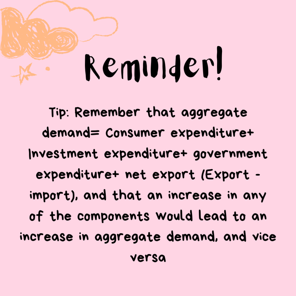
The answer is expansionary fiscal policy! Which is when the government reduces taxation and/or increases government spending to increase aggregate demand.
- Reducing direct taxes (taxes that are imposed on the income or profits of the person who pays it, rather than on goods or services.), increases disposable income of the people (consumers and businesses), this motivates consumer and investment expenditure. And because consumer and investment expenditure are components in aggregate demand, an increase in consumer and investment expenditure leads to an increase in aggregate demand
- Increasing government spending meant that government expenditure increased and an increase in a component in aggregate demand meant that aggregate demand also increased.
How does Fiscal Policy decrease Aggregate demand
The answer is most definitely yes! The government can use contractionary fiscal policy , which is when the government decreases government spending and/or increases taxation to reduce aggregate demand.
- Increasing direct taxes decreases disposable income of the people, reduces consumer and investment expenditure, which will lead to a decrease in aggregate demand.
- Decrease in government expenditure meant that there is a reduction in government spending, which will lead to a reduction in aggregate demand.
How does Fiscal Policy affect the Macroeconomic objectives (Look more forward to this in a future blog)
- Low and stable inflation: By imposing a contractionary fiscal policy the government can reduce demand-pull inflation by reducing aggregate demand which will decrease price level and overall inflationary pressure.
- Low levels of unemployment: By imposing an expansionary fiscal policy, the aggregate demand will increase, which will motivate producers to produce more and this incentivize producers to employ more people, hence reducing unemployment.
- Low levels of poverty: The government can increase government expenditure on unemployment benefits or subsidies, which will increase the income of the impoverished and thus reduces poverty levels in the government expenditure.
- Low levels of income inequality: The government can impose a progressive tax system (A tax rate that increases as income increase) and tax the rich, the additional government revenue can be spent on giving benefits to the poor thus reducing income inequality
- Low sustainable debt: The government can increase its revenue through increased taxation, the increased revenue can be used to repay any fiscal deficit the government has.
Evaluating Fiscal Policy
| Pros | Cons |
| Expansionary fiscal policy can be directed to certain industries through subsidies or tax cuts thus eliminating any private externalities . | Political pressures: politicians may be hesitant to increase taxes in fear of losing the public’s favor. This makes decision making for fiscal policies slow as different politicians may have different views on the economy. |
| The government can earn more revenue through the increased taxation and this increased taxation can be used to spend on other industries or reduce fiscal deficit, helping the country maintain a sustainable debt. | Governments may have to run a budget deficit if large government expenditure is incurred. Funds for subsidies or investments may be taken from budgets of other government activities, this may slow development in other industries as their budgets are reallocated for other purposes (opportunity cost). |
| Contractionary fiscal policy can be directed to industries where the government wants to restrict consumption via an increase in corporate tax or indirect taxation thus reducing any negative externality. | Crowding out: If government attempts to increase spending through increased borrowing they may monopolize the central bank’s money supply causing an increase in interest rate. This increase in interest rate may discourage consumer and investment expenditure, hence aggregate demand may not increase enough to rid a deflationary gap |
| Government spending increases economic development in the long run. Any investment in health care, infrastructure or education will benefit the country’s economic development when these investments are finally built. The funding of these investments also encourages employment to fulfill the investment, so in the long run people will also have more jobs and income thanks to these investments. | The multiplier effect makes it difficult for governments to decide how much they should spend in the economy. As any injection in to the economy will lead to a proportionately larger increase in national income. |
How does Fiscal policy remove Inflationary gap?
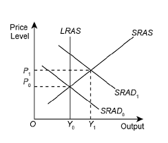
Before the contractionary fiscal policy, the aggregate demand of the economy was at SRAD1 and the short run aggregate supply of the economy was denoted by SRAS curve. They intersect to give the equilibrium price level at P1 and actual output of Y1. The problem is that the actual output is greater than the optimum level of output (Y1 >Y0) and this creates a inflationary gap.
To eliminate the inflationary gap the government increases direct taxation which discourages consumer and investment expenditure, this leads to an decrease in aggregate demand denoted by the shift in SRAD curve from SRAD1 to SRAD0. This leads to a fall in price level from P1 to P0 and an decrease in real GDP from Y1 to Y0 thus eliminating the deflationary gap.
OR
To eliminate the inflationary gap the government decreases its spending which decreases government expenditure, since government expenditure is a component of aggregate demand this leads to an decrease in aggregate demand denoted by the shift in AD curve from AD1 to AD2. This leads to an decrease in price level from P1 to P2 and an decrease in real GDP from Y1 to Y0 thus eliminating the inflationary gap.
How does Fiscal Policy remove deflationary gap?
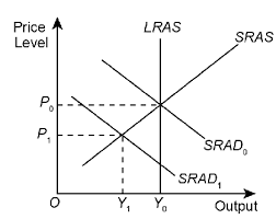
Before the expansionary fiscal policy, the aggregate demand of the economy was at SRAD1 and the short run aggregate supply of the economy was denoted by SRAS curve. They intersect to give the equilibrium price level at P1 and actual output of Y1. The problem is that the actual output is smaller than the optimum level of output (Y1 <Y0) and this creates a deflationary gap.
To eliminate the deflationary gap the government reduces direct taxation which incentivise consumer and investment expenditure, this leads to an increase in aggregate demand denoted by the shift in SRAD curve from SRAD1 to SRAD0. This leads to an increase in price level from P1 to P0 and an increase in real GDP from Y1 to Y0 thus eliminating the deflationary gap.
OR
To eliminate the deflationary gap the government increases its spending which increases government expenditure, since government expenditure is a component of aggregate demand this leads to an increase in aggregate demand denoted by the shift in SRAD curve from SRAD1 to SRAD0. This leads to an increase in price level from P1 to P0 and an increase in real GDP from Y1 to Y0 thus eliminating the deflationary gap.
Higher level Economics: The Multiplier effect
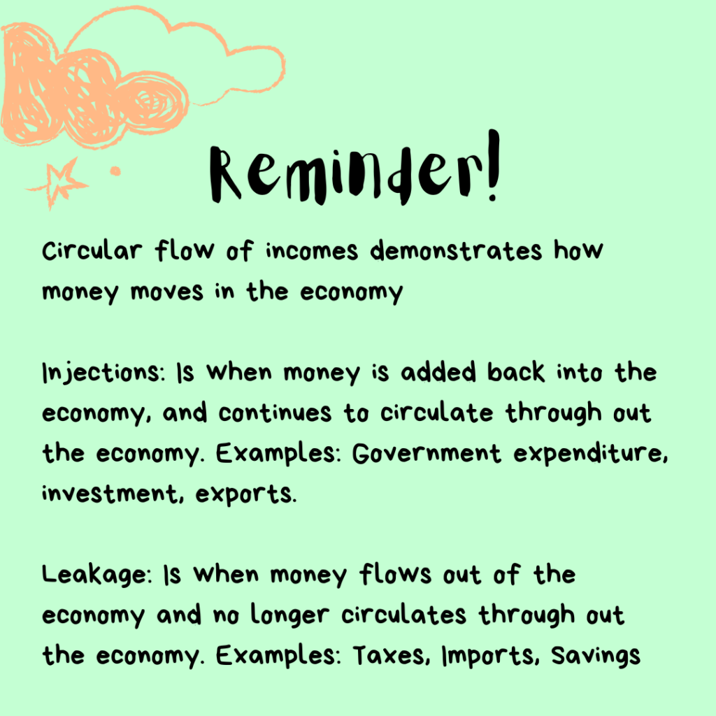
- The multiplier effect: Is the phenomenon that states that any increase in aggregate demand will lead to a proportionally larger increase in national income.
- Government spending and business investments are injections to the circular flow of income and any injections to the circular flow of income are multiplied through the economy as people receive a share of the income and then spend a part of what they will receive. The other part leaks out of the economy.
For example: The government spent $100 million to build a hospital. This $100 million goes to a vast number of people for the factors of production they will provide. The money is income to the builders, architects, engineer, etc who build the hospital. This $100 million also goes to the providers of raw material. The point is this $100 million becomes income to a lot of people.
However, people don’t spend 100% of their income on goods and services. Perhaps 10% goes to taxes, 20% will be saved and 5% goes to imports (imports, taxes, and savings are leakage for the economy), hence 35% will leak out from the economy. This means that the remaining income will be 65% of the income will be spent on goods and services. This is known as marginal propensity to consume (MPC), it is the proportion of an increase in income that gets spent on consumption and this is expressed in decimals. So in this case the MPC is 0.65.
To find out the multiplier in which national income will increase these two formulas can be used
- 1/(1-MPC) or 1/ (MPS+MPM+MRT), where MPS is the marginal propensity to save, MPM is the marginal propensity to import, and MRT is the marginal rate to tax. Both formulas equal to1/ MPW, where MPW stands for marginal propensity to withdraw. (It’s the same as the infinite geometric sequence formula)
So in the example above we can use the first formula to find the multiplier
1/(1-0.65)
=2.8571428571, approximately 2.86
and to find how much this $100million dollars will make in the economy we will simply multiply the multiplier with the amount invested.
So, 2.86* $100 million= $286 million
Sources
- IBDP Economics Textbook
- …and my mind 😉

Hey there, thanks for reading my blog. If you want to read more blogs surrounding Economics, check it out here.
See you! Good luck out there.

