Table of Contents
- 3.2.1 – Aggregate demand
- 3.2.2 – Determinants of the aggregate demand components
- 3.2.3 – Aggregate supply
- 3.2.4 – Macroeconomic equilibrium in the short run
- 3.2.5 – Equilibrium in the long run
- 3.2.6 – Assumptions and implications of the models
3.2.1 – Aggregate demand
Introduction to AD (Aggregate demand)
Imagine everything that’s bought and sold in a country – all the goods and services. Aggregate demand is the total amount people in that country are willing to buy at a particular average price level, at a specific time. So, it’s a big picture of what’s being purchased in an economy.Imagine everything that’s bought and sold in a country – all the goods and services. Aggregate demand is the total amount people in that country are willing to buy at a particular average price level, at a specific time. So, it’s a big picture of what’s being purchased in an economy.
To find out the value of something, like a country’s economy, we use what’s called the expenditure approach. This approach adds up different factors:
- Consumption (C): This is how much people spend on goods and services.
- Investment (I): This includes spending on things like buildings, machinery, and other business investments.
- Government spending (G): This refers to the money the government spends on goods and services.
- Exports minus Imports (X-M): This calculates the difference between what a country sells to other countries (exports) and what it buys from them (imports).
So, to calculate the total value using the expenditure approach, you add up C (consumption), I (investment), G (government spending), and the difference between exports and imports (X-M).
When Aggregate Demand (AD) increases, it means that overall spending in the economy has gone up. This typically happens when people, businesses, or the government are spending more money. When this occurs, it often indicates that the economy is growing. Conversely, if Aggregate Demand decreases, it suggests that spending has gone down, which can indicate a slowdown or contraction in the economy.
Consumption refers to all the money spent by regular people or households on things they buy, like groceries or clothes.
Investment is the total spending by businesses on things like buildings, machinery, or equipment for their operations.
Government spending includes all the money the government spends on various things like paying salaries to public sector employees, funding public services, and investing in infrastructure. It does not include money given out as transfers, like social security payments.
Net exports are the difference between what a country earns from selling goods and services abroad and what it spends on buying goods and services from other countries. Basically, it’s about how much a country sells to other countries minus what it buys from them.
Individuals, businesses, and governments can all be involved in exporting and importing goods and services.
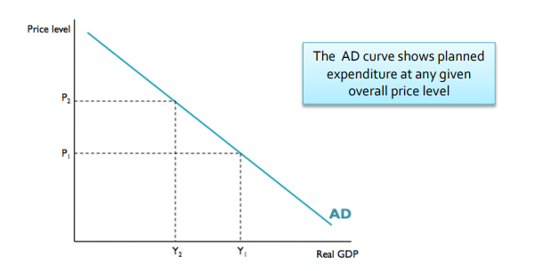
The AD Curve
Source: Study Mind
Real GDP is shown on the x-axis, while the price level is shown in the y-axis.
The Aggregate Demand (AD) curve slopes downwards. This means that when average prices are lower, there tends to be higher demand for goods and services overall. Conversely, when average prices are higher, the demand for goods and services tends to decrease.
Movement along the AD curve

Source: Kognity
When there’s a change in the average price level (AP) in an economy, it causes a movement along the Aggregate Demand (AD) curve. This means that as the average price level changes, the quantity of goods and services demanded also changes, which is reflected in the movement along the AD curve. According to the diagram, when price level decreases, real GDP increases. However when price level increases, real GDP decreases. These are the shifts in the AD curve.
3.2.2 – Determinants of the aggregate demand components
- Consumption is influenced by factors like consumer confidence (how optimistic people feel about the economy), interest rates (the cost of borrowing money), wealth (assets owned by individuals), income taxes (taxes paid on income), household indebtedness (how much debt households have), and expectations about future prices.
- Investment is influenced by factors such as interest rates (the cost of borrowing for businesses), business confidence (how optimistic businesses are about the economy), technology (innovations that can improve productivity), business taxes (taxes paid by businesses), and corporate indebtedness (how much debt companies have).
- Government spending is affected by changes in political and economic priorities. For example, if a government decides to focus more on infrastructure development, it might increase spending in that area.
- Net exports are influenced by factors such as the income of trading partners (how well other countries are doing economically), exchange rates (the value of one currency compared to another), and trade policies (rules and regulations governing international trade).
3.2.3 – Aggregate supply
The actions of businesses spark intense debates in economics. How they decide on prices for resources and goods has big effects on our lives. In microeconomics, we look at how much businesses are willing and able to produce, considering many factors. But in macroeconomics, aggregate supply (AS) is viewed differently based on the time frame. We’ll explore aggregate supply (AS) in both the short and long term for the entire economy.
Aggregate supply in the short-run
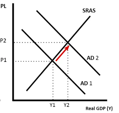
Aggregate supply refers to the total amount of goods and services produced in an economy, known as real GDP, over a certain period at various price levels. In macroeconomics, the short run is the period when resource prices remain relatively stable. Businesses typically don’t encounter frequent changes in costs on a day-to-day or weekly basis to ensure stability. Consequently, there’s a positive connection between the output firms are willing to provide and the selling prices of goods and services. When firms receive higher prices for their products, they become more inclined to produce more, as long as their production costs, especially wages, stay steady in the short run.
Source: EconomicsHelp
In Figure 1, when the price level in the economy rises from P1 to P2, according to the short-run aggregate supply (SRAS) curve, the real GDP or output can increase from Y1 to Y2.
Determinants of SRAS
The aggregate supply curve, much like the supply curve in microeconomics, slopes upward. Shifts in the short-run aggregate supply (SRAS) curve are mainly caused by changes in the costs of factors of production. These changes include:
- Resource prices – If energy prices decrease, the short-run aggregate supply (SRAS) curve will shift to the right because the costs of resources to firms are reduced.
- Government intervention – Regulation, change in tax
- Government subsidies – Governments may offer subsidies to firms to enable them to enhance their productive resources, whether in terms of quality or quantity.
When the SRAS curve shifts to the right, it means firms produce more real GDP at any price level, indicating an increase in short-run aggregate supply. Conversely, when the SRAS curve shifts to the left, it means firms produce less real GDP at any price level, indicating a decrease in short-run aggregate supply.
Other views of aggregate supply
In the long run, all factors of production can be adjusted. The quantity and quality of factors of production available to firms at any given time, rather than production costs, determine how much firms can produce.
Two contrasting schools of thought have different perspectives on the role of government in managing the economy: the ‘new classical’ or ‘monetarist’ school and the ‘Keynesian’ school. Their main disagreement revolves around long-run aggregate supply. We will delve into both of these views below.
New classical
The new classical, or monetarist, school of thought emphasizes the efficiency of the market. As demonstrated in microeconomics, when prices are allowed to adjust freely without price controls, taxes, or subsidies, markets can naturally correct any imbalances. Moreover, at equilibrium, societal welfare is optimized through allocative efficiency.
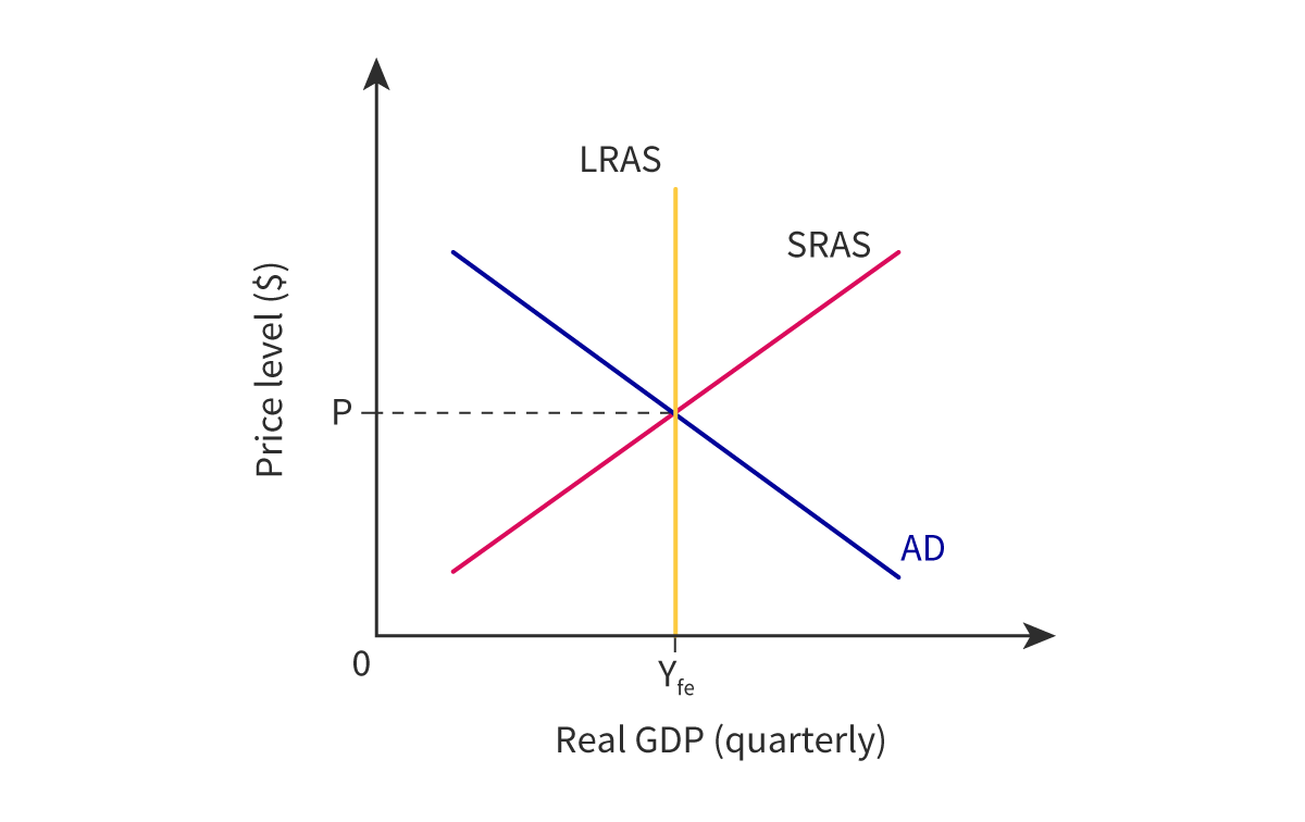
This principle extends to the macroeconomy as well. If resource prices fluctuate according to market forces, then all resources can be fully utilized in the long run, maximizing the nation’s output. The economy will consistently return to its full employment level of output, also known as potential GDP, regardless of the price level’s impact. Hence, we can depict a perfectly inelastic long-run aggregate supply (LRAS) curve.
Source: Kognity
The new classical school posits that in the long run, if prices are completely flexible, the price level doesn’t impact firms’ output levels or profits. Therefore, firms lack the incentive to increase production in the long run. For instance, if the price level decreases and firms can reduce worker wages accordingly, they can maintain the same level of employment and output.
Keynesian view

Source: Kognity
The Keynesian Aggregate Supply (AS) curve is divided into three sections:
- The horizontal section: This represents a period when there is ample unused capacity in the economy.
- The upward-sloping section: Here, although some spare capacity remains, competition for limited resources begins to emerge.
- The vertical section: This indicates full employment in the economy.
During a recession, firms may have no choice but to lay off workers if wages don’t decrease. This is because they sell fewer goods due to low aggregate demand, aiming to maintain profits. This gap between actual output (Y1) and potential output (Yfe) results in unemployment. However, reducing wages is challenging for firms, though not impossible.
Similarly, firms are hesitant to lower prices for their goods and services. They often seek alternative cost-cutting measures to maintain revenue, particularly in severe or prolonged downturns. Only when the economy approaches full employment and resources become scarce do prices begin to rise.
AS and factors of production
While the Short-Run Aggregate Supply (SRAS) curve shifts due to factors affecting production costs, the Long-Run Aggregate Supply (LRAS) represents an economy’s potential production capacity. This capacity is determined by the quantity and quality of a country’s land, labor, and capital.
These terms might sound familiar from previous topics, as they are the factors of production encountered in microeconomics. Similar to the Production Possibilities Curve (PPC), the LRAS also reflects a country’s potential capacity. Both the PPC and LRAS share factors that shift the curves inward or outward, representing changes in the nation’s economic potential.
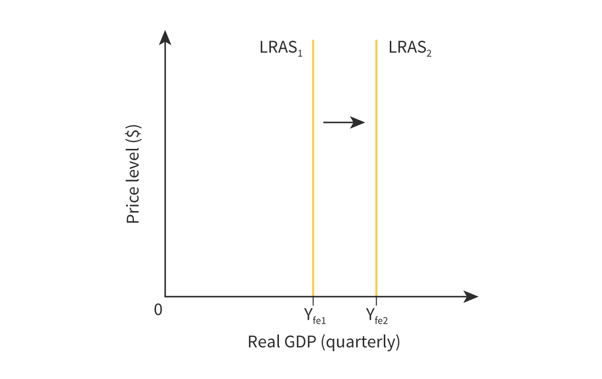
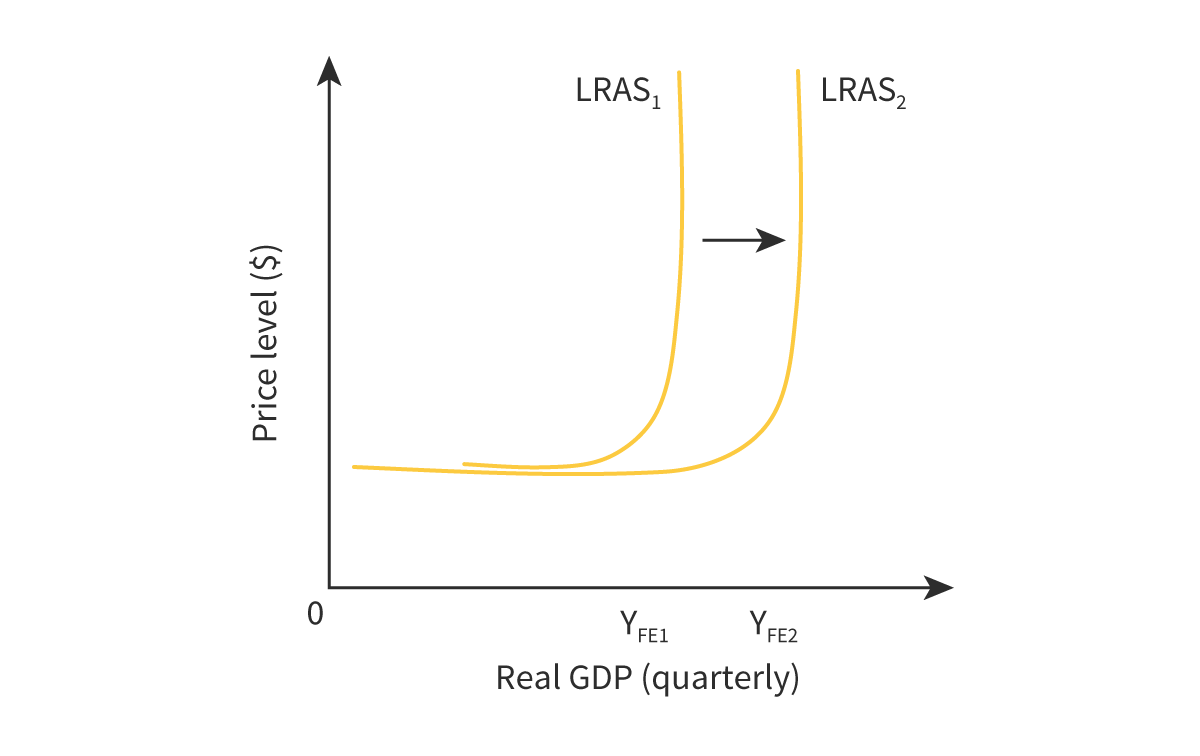
Changes in the quantity or quality of factors of production can shift the LRAS curve. This includes anything significantly affecting land, labor, or capital in an economy. Regardless of whether adopting the new classical or Keynesian view, an increase in the quality or quantity of these factors will shift the LRAS curve outward, enhancing the economy’s potential. Conversely, a decrease in the quality or quantity of these factors will shift the LRAS curve inward.
Land
Land encompasses the natural resources and inputs available within a country. For instance, discoveries of new oil deposits can expand the land factor of production, enhancing the economy’s capacity. Additionally, land can be utilized more effectively or enhanced through technological advancements, such as new methods for utilizing oil efficiently. This improves the quality of available land.
The diagram below shows an increase in the long-run AS.
Source: Kognity
Labor
Labour refers to the individuals comprising the workforce of a country. Increases in immigration or domestic birth rates can augment the quantity of available labour, leading to a larger labor force with the arrival of working-age migrants or the maturation of domestically born individuals. Moreover, labor can be utilized more efficiently or enhanced through improvements in skills or education. This elevation in the quality of labor, often termed “human capital” by economists, leads to a permanent shift in the LRAS curve to the right (outward) as education and training enhance the quality of labor.
Source: Kognity
Capital
Capital encompasses the tools and machinery employed in economic production, including factory machinery or a country’s infrastructure like roads and railways for transporting goods. Enhancing the quantity of capital involves investing in production means, such as constructing more factories or expanding transportation networks. Improving the quality of capital entails enhancing the productivity of existing capital, such as retrofitting a factory to boost energy efficiency or constructing a faster railway system.
3.2.4 – Macroeconomic equilibrium in the short run
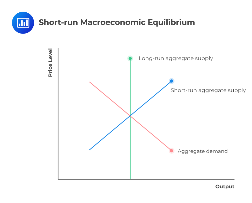
In the short run, equilibrium is established where aggregate demand intersects with short-run aggregate supply.

(Inflationary and deflationary gap) Source: Kognity
Inflationary gap: a reduction in Aggregate Demand (AD) leads to the economy producing below its full employment level, termed a recessionary or deflationary gap. Real GDP falls below potential GDP at Ye.
Deflationary gap: an increase in AD results in real GDP exceeding potential GDP. This situation denotes an inflationary gap, or inflationary pressure, characterized by a rising price level and unemployment below natural rate of unemployment. The economy operates above its full employment level of Ye.
Source: Economics Help
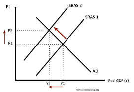
Shifts in Short-Run Aggregate Supply (SRAS) can also impact the short-run macroeconomic equilibrium. SRAS1 shifts leftward due to a supply shock or increased resource prices. Consequently, the economy produces less real GDP, accompanied by a rise in the price level. This scenario, known as stagflation, is highly undesirable as it entails falling GDP, rising unemployment, and increasing prices. Conversely, a rightward shift in SRAS due to changes in its determinants signifies an expansion of real GDP and a decrease in the price level. These short-run fluctuations in Aggregate Demand (AD) and SRAS elucidate the oscillations of the business cycle.
3.2.5 – Equilibrium in the long run
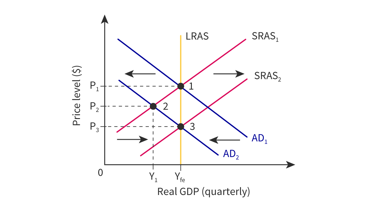
Long-run equilibrium according to new classical model
Aggregate demand falling
Source: Kognity
Above shows an economy returning to full employment equilibrium after a recession, according to the new classical model.
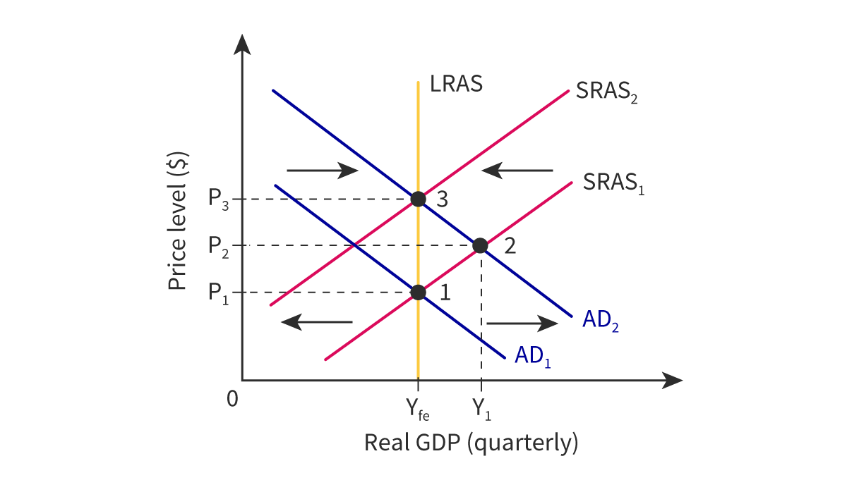
Rising aggregate demand
Source: Kognity
As such, there are only short-run fluctuations in output, but the economy will return to the full employment level of output in the long run. Therefore, the new classical perspective advocates a focus on the long-run potential of the economy. This is particularly true in the case of rising aggregate demand, as the short-run increases in output will not hold. Economists who subscribe to this school of thought will want the government to invest in education and infrastructure to boost the productive potential of the economy and shift long-run aggregate supply outwards. The short-run fluctuations in the economy will not affect the real GDP but will only result in increases in the price level.
Long-run equilibrium according to the Keynesian view
The Keynesian theory emerged as a response to the failure of economies to self-correct during the Great Depression, contrary to the beliefs of the new classical theory. Despite the prevailing notion that economies would naturally gravitate towards full employment, the prolonged depression prompted a reevaluation of this idea. John Maynard Keynes introduced his influential work, “The General Theory of Employment, Interest, and Money,” in 1936, recognizing the need for government intervention in the short run to address economic challenges.
The crux of disagreement stems from the assumption that resource prices would decrease in a deflationary environment. Keynes advocated for increased government spending to stimulate the economy, challenging the notion that prices always adjust downward. He argued that factors such as employment contracts, minimum wage laws, and trade unions could prevent prices from declining as expected. Keynes suggested that economies could become “stuck” in a short-run position and fail to return to full employment levels of output without government intervention.
Source: Kognity
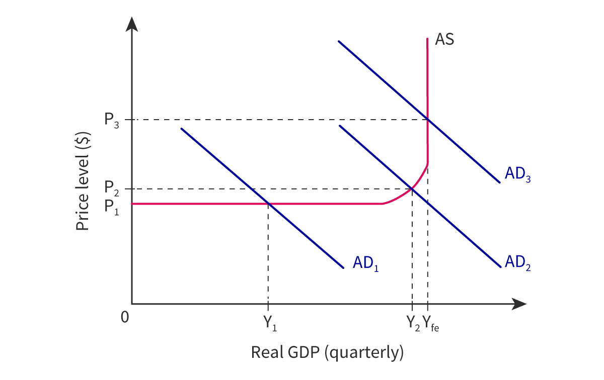
The graph above shows the AD and AS curves in Keynesian view.
According to Keynes, the economy can reach equilibrium below the full employment level of output and remain in that state until government intervention occurs. This scenario, known as a deflationary or recessionary gap, occurs when both the price level and real GDP decrease due to a leftward shift of Aggregate Demand (AD). In Figure 4, this situation corresponds to aggregate demand being at AD1, resulting in a real output of Y1 and a price level of P1, indicating lower real GDP and price level compared to AD3 at full employment. Keynes believed that economies could become stuck at Y1 unless government spending intervened. Only when aggregate demand increases to AD2 does upward pressure begin to build on the price level.
Thus, according to Keynesian economics, the economy can remain at Y1, below the full employment level of income, which is also regarded as equal to the natural unemployment rate by economists. Consequently, the unemployment rate will be significantly higher than the natural rate of unemployment.
As resources become more fully utilized, the redistribution of resources from one use to another typically occurs through price increases. In the labor market, a shortage of workers prompts firms to compete for existing workers by offering higher wages. This increase in wages leads firms to raise the prices of goods and services they offer, causing the average price level to rise across the economy.
When the economy reaches this stage, the government should focus on investing in the long-term potential of the economy.
3.2.6 – Assumptions and implications of the models
| Keynesian | New classical | |
| Markets | Some markets can remain in a state of disequilibrium for extended periods of time | Disequilibrium is resolved by the actions of market forces |
| Unemployment | Long-term unemployment should not be tolerated as it diminishes economic potential | A sign that the market for labour is in disequilibrium |
| Wages | Wages are “sticky” | Trade unions and minimum wages can impede the labor market’s ability to achieve equilibrium |
| Role of government | Imperative for the government to intervene with increased spending, even if it means borrowing funds | Support markets, allow them to return to equilibrium. |
| View of borrowing | Minimize the phenomenon of crowding out during a recession | Government borrowing during recessions can potentially crowd out private investment |
Government’s role in the economy
New classical economists advocate for limited government intervention in markets, particularly regarding prices and resource allocation. While they acknowledge the importance of addressing externalities and ensuring worker safety, they believe that prices enable markets to self-correct during recessions. Consequently, they argue that the government’s role should primarily involve reducing market restrictions and implementing supply-side policies. These policies aim to enhance the aggregate supply of the economy by promoting business investment, production, growth, and reducing unemployment. This is achieved by fostering growth through increasing both the quantity and quality of factors of production. However, the success or failure of such policies implemented by governments worldwide in the past decade remains a subject of debate.
And that’s it for Topic 3.2! See you in the next revision guide!
Psst! Check out all of our Economics revision guides here!
Sources:
Study Mind
EconomicsHelp
